jatinhans.com / lab · Case study · Currency forecasting
Which currency questions are actually answerable?
Ten years of daily prices for the euro, the yen and the rupee against the dollar. Three questions, the same data, every answer scored against a simple guess I named first. Two of the three were dead ends. The third fixes a number companies set every month.
Every input is lagged one trading day and matched to its question’s frequency. Models are scored only on data they never saw. Method in section 07, sources in the appendix.
01 · The shape of the problem
The market hides which way it will move. It telegraphs how rough the ride will be.
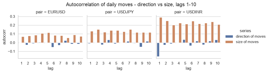
Before building anything, ask the price history one question: does what happened over the last few days tell you anything about today? Ask it twice. Once about the direction of moves, once about their size.
Source: notebooks/01_direction.ipynb
The blue bars sit at zero on every pair. Yesterday’s direction tells you nothing about today’s. One bar on the rupee panel does dip below zero, since the rupee tends to give back a little the day after a move, but it is too small and too short-lived to build on. The models confirmed that later. The orange bars run clearly positive everywhere: wild days follow wild days, calm days follow calm days.
That single difference decides all three verdicts below. Q1 has no answer in this data. Q2 and Q3 do.
02 · Q3 · Planning rate
Plan next month around today’s rate, not last month’s average
Businesses need one exchange rate agreed in advance: a budgeting rate, a pricing rate, or a rate written into a contract. What that number is really guessing at is next month’s average rate. Almost nobody tests it as its own question.
We compared three ways of setting it at every month-end across 104 months, 2017 to 2026. Score it by asking how far off the guess was, on average, as a percentage of the average that actually happened. Smaller is better.
Average miss, %. 104 months per pair, lower is better
A · last month’s average B · today’s rate C · small statistical model
Guess C, the statistical model, ties guess B on every pair. The win comes from a better starting point. The modelling adds nothing. The whole test fits in a few lines: at each month-end, record what each method would have guessed, then compare it with the average that actually happened.
Source: scripts/14_period_average.py, condensed
At each month-end, set the planning rate from today’s rate instead of last month’s average.
No model to deploy and no data to buy. It held on all three pairs tested.
03 · Q2 · Roughness
Size is forecastable where direction is not
“Volatility” just means how much the price jumps around. A calm week versus a wild one. Knowing next week will be wild says nothing about which way prices go, but it does tell a business how much safety margin to leave.
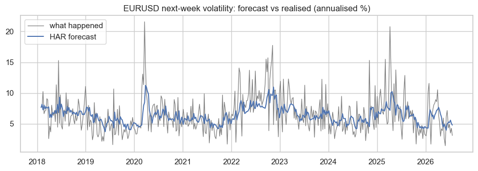
Two forecasters raced each other one week ahead, over 426 separate weeks per pair. The do-nothing guess assumes next week is as wild as the recent past. The volatility model is a textbook recipe called HAR. It blends yesterday’s choppiness with last week’s and last month’s, weighting each by what has worked historically.
Source: scripts/10_turbulence_har.py, condensed
The model cuts forecast error roughly in half on every pair, 51-57% less, measured by the scoring rule statisticians use for volatility forecasts. That rule punishes under-warning about a storm harder than over-warning about one.
Source: scripts/10_turbulence_har.py
Next-week forecast error. 426 weeks per pair, lower is better
| Pair | Forecaster | Error score | vs do-nothing |
|---|---|---|---|
| EURUSD | Do-nothing guess | 0.84 | baseline |
| Volatility model (HAR) | 0.36 | 57% less error | |
| HAR + machine learning | 0.42 | worse than HAR alone | |
| USDINR | Do-nothing guess | 1.72 | baseline |
| Volatility model (HAR) | 0.84 | 51% less error | |
| HAR + machine learning | 0.99 | worse than HAR alone | |
| USDJPY | Do-nothing guess | 1.13 | baseline |
| Volatility model (HAR) | 0.55 | 51% less error | |
| HAR + machine learning | 0.66 | worse than HAR alone |
Error score is the volatility scoring rule described above. Units matter only for comparison. Monthly results in A.3.
Look at the third row of every block. Stacking machine learning on top of the simple recipe made forecasts worse every time at this horizon. The extra complexity cost accuracy and bought nothing.
This tells you how much cushion to leave, and nothing about which way the rate moves. In a week forecast to be wild you buy protection sooner and price in a bigger buffer. Put less at stake. In a week forecast calm, run the reverse.
04 · Q1 · Direction
Nothing beat “the next period repeats the last one”
Fifteen approaches were graded on direction: classic trading rules, statistical models, machine-learning models, and combinations of all three. Every one raced the laziest guess available. Assume the next period does what the last one did.
Accuracy is scored out of 100, so “+6.4” means the best model was right about six more times per 100 guesses than the lazy one. Every advantage here came in smaller than the uncertainty around it. Any of them could be luck.
Extra correct guesses per 100 vs lazy guessing. 322 predictions per pair, final unseen test period
| Pair | Extra correct | Could it just be luck? |
|---|---|---|
| EURUSD | +6.4 | Yes, too close to call |
| USDJPY | +1.6 | Yes, too close to call |
| USDINR | +1.4 | Yes, too close to call |
A model can look fine on accuracy and still be dangerously overconfident
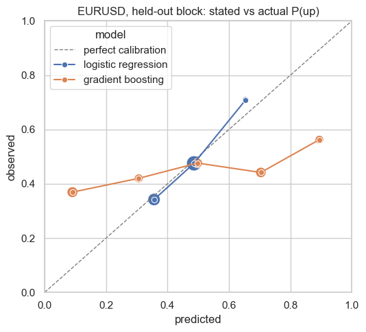
Some models state a confidence with every guess (“70% sure it goes up”). We checked whether those confidences are honest: when a model says 70%, is it right about 70% of the time?
Source: notebooks/01_direction.ipynb
Logistic regression sits near the line, so its stated confidence means something. Gradient boosting is far off it. When it claimed “90% sure” it was right barely half the time. If you act on a stated probability, this chart matters more to you than any accuracy table.
The Fed’s words measure cleanly and add nothing
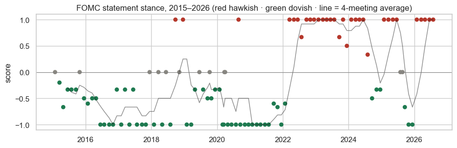
The second dead end got tested rather than assumed. All 99 FOMC statements were scored hawkish to dovish by counting phrases, a method any reader can check. The scorer passes its sanity check: the 2022-23 rate-hike era reads hawkish, the 2020 emergency cuts read dovish.
Source: scripts/12_stance_score.py · scoring method and full numbers in A.4
Fed into the models across the same 402 weeks, the scores changed nothing. The input was rejected. The experiment stays in the repo as a documented negative, because a measurement can be valid and still add no forecasting value, and both halves of that are worth publishing.
05 · The most transferable result
When a forecast looks too good for its field, audit the timestamps first
Early on, one model looked 70% accurate at predicting the next day. Implausibly good. The cause was a timestamp mismatch: Yahoo stamps its currency prices earlier in the day than it stamps the dollar index. Join the two on the same date and “today’s” dollar move quietly carries information about tomorrow’s euro move. The model was peeking.
The check that caught it uses correlation, a score from −1 to +1. Near 0 means no connection. Near −1 or +1 means strongly connected.
Source: notebooks/01_direction.ipynb, section 1
After the one-day shift, the 70% “accuracy” collapsed to ordinary guessing. Every number on this page comes from the fixed data. Of everything in this project, finding that bug is the part most likely to be useful to someone else.
06 · The close
What ten years of public data rules out, and what it supports
Rate-direction inputs
Ten years of public data give no reliable basis for a “the rate will move this way next” prediction at day, week or month horizons. Worth knowing before it reaches a roadmap.
Roughness-aware planning
Forecast the size of the moves and let that set your buffers and your limits. It is the part of the problem public data actually answers.
Free data, open tools
Every result here comes from public sources and open-source tooling, and reruns from the repository. Ruling something out this cheaply was worth the time on its own.
07 · How it was tested
Baselines named before models were built
A named “lazy guess” for every question
Repeat-the-last-period for direction, assume-it-continues for roughness, carry-forward for the planning rate. Beat the lazy guess or it doesn’t count. Half of what this study found came from fixing the comparison rather than the model.
No peeking, enforced in code
Every input is shifted one trading day. Daily data predicts the next day, weekly the next week, monthly the next month. Models slide forward through time and are scored only on data they have never seen. Mixing frequencies is where accidental peeking usually creeps in.
Uncertainty stated on every claim
Every headline number carries a statistical uncertainty range and its sample size. Where the sample is small, I call the result an anecdote.
Confidence scored, not assumed
Stated probabilities are graded against reality. Overconfident models get their confidence corrected using data they haven’t seen, or are shown as-is with a warning attached.
Fully reproducible
Data, pipeline, models and every chart on this page regenerate from the repository. Two notebooks tell the story end to end, and numbered scripts rebuild every table.
Appendix
Detail, caveats and what sits behind the summary
A.1 sources · A.2 planning-rate table · A.3 monthly roughness · A.4 Fed language · A.5 limits · A.6 repository
A.1 - Inputs, sources and coverage
Nothing here is proprietary or paid. That is deliberate: it shows what currency forecasting can deliver before anyone spends money on data. Coverage gaps are stated rather than papered over.
| Input | What it captures | Source | Coverage |
|---|---|---|---|
| Daily prices | Closing price for each pair, back to 2015 (the first year warms up the calculations) | Yahoo Finance | All 3 pairs |
| Recent moves | The last move plus how far the price travelled over 1, 3, 6 and 12 months | Derived | All 3 pairs |
| Choppiness | How much the price has been jumping around, over short, medium and long windows | Derived | All 3 pairs |
| Market backdrop | Moves in the dollar index and the VIX, a widely used market-nervousness gauge | Yahoo Finance | All 3 pairs |
| Interest-rate gap | The difference between what each currency earns in interest | FRED | All 3 pairs |
| Fund positioning | Whether large funds are betting for or against the euro and the yen, reported weekly | CFTC | No rupee version exists |
| Policy language | 99 statements from the Fed’s rate-setting committee, scored hawkish to dovish | US Federal Reserve | Dollar side only |
A.2 - The planning-rate comparison in full
The three methods scored side by side. Guess C ties guess B on every pair, which is why the body section shows the comparison as bars rather than a table.
| Pair | A · last month’s avg | B · today’s rate | C · model | B vs A |
|---|---|---|---|---|
| EURUSD | 1.21 | 1.01 | 1.03 | −16% |
| USDINR | 0.90 | 0.66 | 0.65 | −28% |
| USDJPY | 1.51 | 1.13 | 1.14 | −25% |
Average miss as a % of the average that actually happened. 104 months per pair, lower is better.
A.3 - Roughness at the monthly horizon
The weekly result is the headline because it is the horizon most decisions run on. The monthly horizon has a smaller sample and a less clean story: the simple model still wins on two pairs, the machine-learning variant narrowly takes the rupee, and all the gaps are smaller.
| Pair | Forecaster | Error score |
|---|---|---|
| EURUSD | Do-nothing guess | 0.181 |
| Volatility model (HAR) | 0.153 | |
| HAR + machine learning | 0.219 | |
| USDINR | Do-nothing guess | 0.626 |
| Volatility model (HAR) | 0.488 | |
| HAR + machine learning | 0.465 | |
| USDJPY | Do-nothing guess | 0.335 |
| Volatility model (HAR) | 0.259 | |
| HAR + machine learning | 0.370 |
97 months per pair, same error score as the weekly table, lower is better. One caveat on measurement: roughness is estimated from end-of-day prices. Minute-by-minute data would measure it more precisely and wasn’t available, so the claims are kept proportionate to that.
A.4 - The Fed-language method and numbers
A transparent dictionary method: count phrases, so any reader can check why a statement scored the way it did.
The direction models were run with and without these inputs on the same 402 weeks. One note so the numbers don’t surprise you: these are three-way guesses, up or down or roughly flat, so random guessing scores about 33%. Numbers below 50% are normal here.
| Model | Without, % | With, % | Verdict |
|---|---|---|---|
| Logistic regression | 39.6 | 38.1 | No measurable effect |
| Gradient boosting | 42.5 | 43.8 | No measurable effect |
Accuracy barely moved, and it moved in opposite directions for the two models. The uncertainty around both differences includes zero.
A.5 - Known limits of this study
- -Three pairs only, two heavily traded and one from a developing economy. Don’t assume the findings carry to other currencies
- -Roughness is estimated from end-of-day prices rather than measured minute by minute
- -No rupee version of the fund-positioning data exists, so USDINR sits that input out
- -Central-bank language covers the Fed only. The Indian central bank’s statements were not machine-collectable
- -No transaction costs are modelled. This measures forecast quality, and says nothing about whether a trading strategy would clear costs
A.6 - What is in the repository
- -Two notebooks that tell the whole story. Direction end to end, then roughness, the planning rate and the Fed-language experiment
- -The full bench of fifteen direction models, including classic institutional and retail trading rules, each with its own scorecard
- -All raw data committed, so everything reruns offline. An offline validator checks every stored file
- -Every table and chart on this page, regenerable from numbered scripts